Case Study – Strategies for Uncertainty

18. July 201313. April 2018

On Forecasting New Product Sales, Experience, Artificial Intelligence and Statistics

Forecasting sales for new products is among the most difficult tasks in planning. There is nothing to extrapolate, and in the early stages, there is not even a finished product to present to customers and get their feedback. At the same time, sales forecasts for product innovations are inevitable. Some innovators say they cannot forecast, some say the do not forecast, but in the end, who doesn’t calculate sales forecasts explicitly will do it somewhere, somehow implicitly, often in a less thoughtful and therefore less careful way.

For the following case study, let us assume we are in an innovation-driven industry, which regularly develops new products. The current sales forecasts for product innovations have been done based on model assumptions and market research. Controlling has shown significant, unexplained discrepancies between planning and actual sales developments.

There is a variety of methods available to forecast product innovation sales. For development products that are advanced enough to be presented to potential customers, conjoint analysis offers a tool to gauge perceived product advantage. While that product advantage is quite useful to determine what might be seen as a fair price, its connection to the achievable market share is obvious as a fact but not trivial in numbers. The Dirichlet Model of Buying Behavior links market penetration to market share and can thus be used to estimate the impact of marketing activities. It assumes market shares to be constant over the relevant period of time, but appears sufficiently tested to be considered valid at least for the peak market share to be reached by a product. Regarding the development of market share over time, the Fourt-Woodlock model differentiates between product trials and repeat purchases, whereas the Bass diffusion model describes the early phases of a product lifecycle in more mathematical terms, claiming to model the share of innovators and imitators among customers. For high repeat purchase rates and a vanishing share of imitators, both models are more and more similar.

The problem with all of these models is that in spite of all their assumptions, they still contain quite a few free parameters. In practical use, these parameters have to be derived from market research, taken from textbooks or guessed, introducing a significant degree of arbitrariness into the forecasts. The problem becomes apparent in this quote attributed to mathematician John von Neumann: “With four parameters I can fit an elephant, and with five I can make him wiggle his trunk.” In fact, we will do just that, and the trick will be to find the proper elephant.

A totally different approach from these models would be to go by experience. What has been true for previous product launches, by one’s own company or by others, should have a good chance of being true for for future new products. Obviously, while having personal experience with the introduction of new products will help in managing such a process, a realistic forecast will have to be based on more than the experience of a few products and, therefore, individual managers. Individuals tend to introduce various kinds of bias in their judgements, which makes personal experience invaluable for asking the right questions but highly problematic for getting unbiased, reliable answers.

On the other hand, there is usually plenty of “quantitative experience” available. The company will have detailed data about its own product launches in the target market and in similar markets, and market research should be able to provide market volumes and market shares for competitors’ past innovations. Aligned, scaled to peak values and visualized in a forecast tool, the market share curves from past data could, for example, look like this:

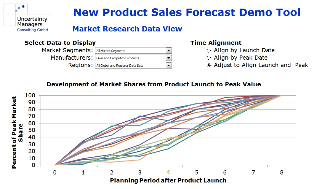
The simplest way to estimate new product sales would be to find a suitable model product in past data and assume the sales of the new product will develop in roughly the same way. That is relatively close to what an experienced individual expert asked for a judgement would probably do, with or without realizing it. Unfortunately, this approach can be thwarted by a variety of factors influencing the success of new products:

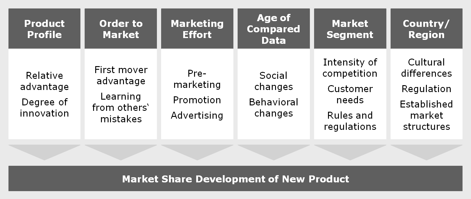
The varying influence of all these factors will make it, at best, difficult to find and verify a suitable model in past data. Besides, judging from one model product yields no error bars or other indication of the forecast’s trustworthiness.

Apparently, to get a reasonable forecast, we need a more complex system, which should be able to learn from all the experience stored in past data. The term “learn” indicates artificial intelligence, and in fact, AI tools like a neural network could be used for such a task: It could be trained to link resulting sales or market share curves to a set of input parameters specifying the mentioned influences. The disadvantage of a neural network in this context is that the way it reaches a certain conclusion remains largely intransparent, which will not help the acceptance of the forecast. Try explaining to your top-level management that you have reached a conclusion with a tool without knowing how the tool came to that conclusion.

On the other hand, there is no need to model a new product exclusively from past data without any further assumptions. All the more analytical models and forecast tools cited above have their justification, and they define a well-founded set of basic shapes, which sales of new products generally follow. New product market shares will usually rise to a certain peak value in a certain time, after which they will either decrease or gradually level off, depending on market characteristics. The uptake curve to the peak value will be either r- or s-shaped, and can usually be well fitted by adjusting the parameters of the Bass model. The development after the peak is usually of lesser importance and depends strongly on future competitor innovations, which are more difficult to forecast. Often, relatively simple models will be able to describe the data with sufficient accuracy – if they use the right parameters.

Generally, all published sales forecast models use market research data from actual products to verify their validity and to tune their parameters. The question is to what extent that historical data actually relates to the products and markets we want to forecast. In this case, we are simply using model parameters to structure the information we will derive from recent market data from our own markets. Based on an analysis of the available data, we have selected the following set of parameters to structure the forecast:

Peak market share
Time from product launch to peak market share
Bass model innovation parameter p
Bass model imitation parameter q
Post-peak change rate per time period

The list may look slightly different depending on the market looked at. Tuning these parameters to the full set of the available data would lead to the average product. On the other hand, we have to take into account the influencing factors displayed in the graph above. These influencing factors can be quantified, either as simple numbers by scoring or by their similarity to the new product to be forecasted. This leads us to the following structure of influence factors, forecast parameters and forecasted market share development:

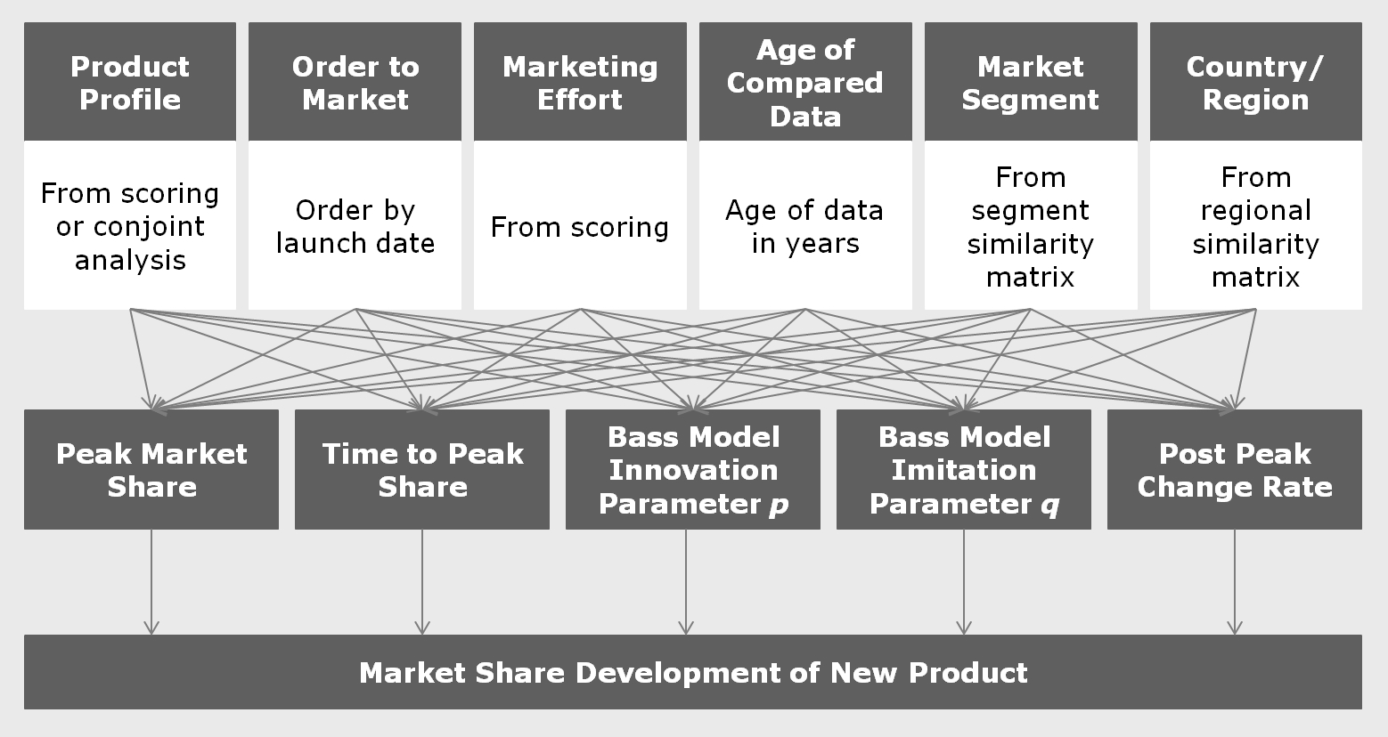
If the parameters were discrete numbers, this graph would describe a Bayesian network. In that case, forecasting could take the form of a probabilistic expert system like SPIRIT, which was an interesting research topic in the 1990s.

In our case, however, the parameters are continuous functions of all the influencing factors, which we approximate using simple, mostly linear, dependencies. These approximations are done jointly in a multidimensional numerical optimization. For example, rather than calculating peak market share as a function of product profile scoring, everything else being equal, we approximate it as a function of product profile, order to market, marketing effort and the other influencing factors simultaneously. The more market research data is available, the more detailed the functions can be. For most parameters, however, linear dependencies should be sufficient. As the screenshot from the case study tool shows, the multidimensional field leads to reasonable results, even if research data is missing in certain dimensions (right hand side graph).

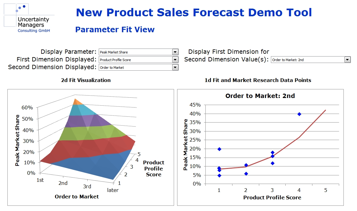
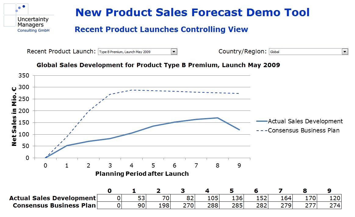
In addition, confidence intervals can be derived in the fitting process, leading to a well-founded, quantitative market share forecast implemented in an interactive model that can be used for all new products in the markets analyzed. Implemented in a planning tool, forecasts from that model could look as follows:

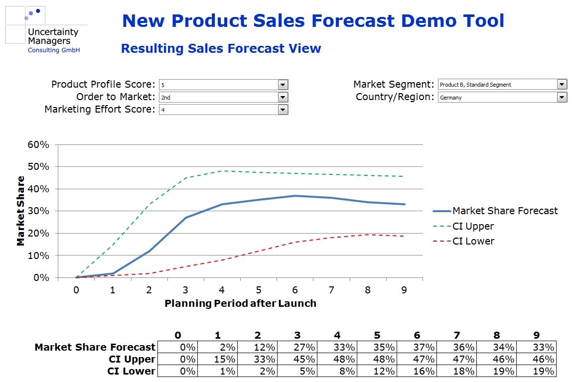
Forecast numbers will depend on the values of the different influence factors selected for the respective product innovation.

This approach presented can be implemented for a multitude of different markets and products, provided there is sufficient market research data available. While using known and well-researched models to structure the problem, the actual information used to put numbers in the forecast stems entirely from from sales data on actual, marketed products. Besides this pure form, it can also be combined with more theory-based approaches, depending on the confidence decision makers in the company have in different theories.

Dr. Holm Gero Hümmler
Uncertainty Managers Consulting GmbH

10. April 201313. April 2018

Bayes’ Theorem and the Relevance of Warning Signs

One of the interesting things about working in the field of business strategy is that the most inspiring thoughts relevant for one’s work are usually not found in textbooks. Dealing with spaceflight, science fiction and fringe technology, the io9 portal is about as geeky as they come and can hardly be considered typical manager’s reading. It does, however, contain fascinating ideas like this one: How Bayes’ Rule Can Make You A Better Thinker. Being a better thinker is always useful in strategy, and the article points out a number of interesting thoughts about how what we believe to be true is always uncertain to a degree and about the fallacies resulting from that. Unfortunately, it just very briefly skips over what Bayes’ Theorem actually says, although that’s really not that difficult to understand and can be quite useful, for example in dealing with things like warning signs or early indicators.

Obviously, Bayes’ Theorem as a mathematical equation is based on probabilities, and we have pointed out before that in management, as in many other aspects of real life, most probabilities we deal with can only be guessed. We’re not even good at guessing them. Still, the theorem has relevance even on the level of rough estimates that we have in most strategic questions, and in cases like our following example, they can fairly reasonably be inferred from previous market developments. Bayes’ Theorem can actually save you from spending money on strategy consultants like me, which should be sufficient to get most corporate employees’ attention.

So, here is the equation in its simplest form and the only equation you will see in this post, with P(A) being the probability that A ist true and P(A l B) being the probability that A is true under the assumption that B is true. In case you actually want more math, the Wikipedia article is a good starting point. In case that’s already plenty of math, hang in there; the example is just around the corner. And in case you don’t want a business strategy example at all, the very same reasoning applies to testing for rare medical conditions. This equation really fits for a lot of cases where we use one factor to predict another:

What does that mean? Suppose we have an investment to make, maybe a product that we want to introduce into the market. If we’re in the pharmaceutical business, it may be a drug we’re developing; it can also be a consumer product, an industrial service, a financial security we’re buying or real estate we want to develop. It may even be your personal retirement plan. The regular homework has been done, ideally, you have developed and evaluated scenarios, and assuming the usual ups and downs, the investment looks profitable.

However, we know that our investment has a small but relevant risk of catastrophic failure. Our company may be sued; the product may have to be taken off the market; your retirement plan may be based on Lehman Brothers certificates. Based on historical market data or any other educated way of guessing, we estimate that probability to be on the order of 5%.

That is not a pleasant risk to have in the back of your head, but help is on the way – or so it seems. There will be warning signs, and we can invest time and money to do a careful analysis of these warning signs, for example do a further clinical trial with the drug, hire a legal expert, market researcher or management consultant, and that analysis will predict the catastrophic failure with an accuracy of 95%. A rare event with a 5% probability being predicted with a 95% probability means that the remaining risk of running into that failure without preparation is, theoretically, 0.25%, or, at any rate, very, very small. The analysis of warning signs will predict a failure in 25% of all cases, so there will be false warnings, but they are acceptable given the (almost) certainty gained, right? Well, not necessarily. At first glance, the situation looks like this:

If we have plenty of alternatives and are just using our analysis to weed out the most dangerous ones, that should do the job. However, if the only option is to do or not do the investment and our analysis predicts a failure, what have we really learned? Here is where Bayes’ Theorem comes in. The probability of failure, P(A), is 5%, and the probability of the analysis giving a warning, P(B), is 25%. If a failure is going to occur, the probability of the analysis predicting it correctly, P(B l A), is 95%. Enter the numbers – if the analysis leads to a warning of failure, the probability of that failure actually occurring, P(A l B), is still only 19%. So, remembering that all our probabilities are, ultimately, guesses, all we now know is that the negative result of our careful and potentially costly analysis has changed the risk of failure from “small but significant” to “still quite small”.

If the investment in question is the only potential new product in our pipeline or the one piece of real estate we are offered or the one pension plan our company will subsidize, such a result of our analysis will probably not change our decision at all. We will merely feel more or less wary about the investment depending on the outcome of the analysis, which raises the question, is that worth doing it? As a strategy consultant, I am fortunate to be able to say that companies will generally just spend only about a permill of an investment amount on consultants for the strategic evaluation of that investment. Considering that a careful strategic analysis should give you insights beyond just the stop or go of an investment, that is probably still money well spent. On the other hand, additional clinical trials, prototypes or test markets beyond what has to be done anyway, just to follow up on a perceived risk, can cost serious money. So, unless there are other (for example ethical) reasons to try to be prepared, it is well worth asking if such an analysis will really change your decisions.

Of course, if the indicators analyzed are more closely related to the output parameters and if the probability of a warning is closer to the actual risk to be predicted, the numbers can look much more favorable for an analysis of warning signs. Still, before doing an analysis, it should always be verified that the output will actually make a difference for the decisions to be made, and even if the precise probabilities are unknown, at least the idea of Bayes’ Theorem can help to do that. Never forget the false positives.

Dr. Holm Gero Hümmler
Uncertainty Managers Consulting GmbH

17. July 201213. April 2018

The Role of Databases for Strategic Planning – Case Study in Palo/Jedox

After discussing the general capabilities and limitations of databases for strategic planning in The Role of Databases for Strategic Planning – Some General Remarks, we have looked at a case study in a relational database accessed through a special data mining tool: The Role of Databases for Strategic Planning – Case Study in Qlikview/Oracle. In this case, we will look at a case study very similar in the business perspective, but based on a different database concept. The database we will be looking at is Palo or Jedox (all product names mentiones are trademarks of the respective owners), accessed not through an external tool but through the database’s standard access mechanisms. Palo is an open source OLAP database, with an upgraded version under commercial license sold under the manufacturer’s name, Jedox. The case study was done using the latest open source version, Palo 3.1.

Again, we are addressing the issue that a planning database will generally contain input from very different people in different parts of the company, and possibly even from outside partners. Large planning databases may contain some replies to “what-if” questions, but discussing and testing the implications of a large number of future developments with so many contributors will usually be impractical. In most cases, information contributors from local marketing or external market research companies will not have enough time to contribute for extended strategic work. Therefore, it will be necessary to use the multitude of planning figures in the database as the basis for a calculation of scenarios and strategic options defined and evaluated later, at the corporate strategy level.

As in the Oracle/Qlikview example, the case study involves a manufacturer of electronic components, systems and services, operating in different regions with a number of product lines. The existing planning database contains basic sales and cost figures for own products and only sales data for the main competitor products or local competitor groups. Planning figures cover some years of back data plus four years of forecast. For the case study, we assume that all the data ist stored in one database cube. That is not the most efficient way of storing the data, as zeros will be stored for competitor cost data, but probably a realistic way such databases will have been set up for reasons of simplicity. Considering the limited data volume of 60 products in 32 regions for seven years, memory will hardly be a serious matter of concern in this case, anyway. The dimensions of the case study cube are product, region, year and figure (the figures being units sold, net revenue, direct cost and overhead cost).

As we will be using a standard Palo user interface, it will be fairly simple to write data back to the database. Therefore, calculated simulation results can be stored in the database as well, in a different cube to keep them separate from data accessed by other users. The new cube has the simulated business case as an additional dimension, the year dimension is extended by the extrapolation, and the figure dimension stores additional figures calculated in the course of the simulation. A plain database access screen, therefore, looks as follows (original forecast db on the top, simulation db on the bottom, click to enlarge):

The first question to answer in accessing data from a Palo/Jedox database is the interface platform to be used. There are two main data interfaces provided: One is Palo Web, a browser-based data access and manipulation tool that also allows calculations and macros, the other comes in the form of plugins for either MS Excel or OpenOffice Calc. The plugins allow simple access from both tables and macros to the data, which can then be manipulated using the full functionality of the respective program. As OpenOffice is less common in companies, the respective plugin was not tested for this case study.

In determining which solution works best for the simulation, we have to keep in mind which tasks will have to be performed by the tool. The simulation has to access relatively large amounts of data simultaneously, then perform complex calculations based on interactive assumptions. Most of the calculations will have to be done in macros.

With the Palo Excel plugin, a set of almost identical database access functions can be performed either in table cells when a table is recalculated or directly from a macro. As accessing many adjacent database entries from a table can be done simultaneously in an optimized way, this form of db access is much faster than from the macro. In fact, reading the whole data volume characterized above into a table is a matter of seconds. Table recalculation has to be set to manual and managed by macros after that to keep the tool performing at reasonable speed, but that can be done quickly and almost invisible to the user. Once the data is in Excel, the respective table can be copied to a Visual Basic array. The fast Visual Basic compiler with reasonable editing and debugging support allows the convenient development of all necessary macros. Running the extrapolation to the simulation timeframe or an interactive simulation in the described manner, writing the data back to Excel tables and updating the respective displays and graphs is a matter of less than five seconds for our example and thus easily fast enough for interactive work. Writing the calculated data back to the database takes a few minutes, as the writing, as opposed to reading data from the database, has to be done cell by cell. This step can therefore not be part of the regular interactive work, but should rather be offered as a possibility of storing the results at the end of an interactive session.

Palo Web provides a table calculation tool similar to Excel or OpenOffice Calc in a browser window:

Palo Web files are stored on the server rather than locally, which may be interesting if they are to be accessed by several users. Cell manipulation and data visualization capabilities are quite similar to Excel and relatively easy to adjust to, but have their peculiarities and restrictions in some details. The database access functions themselves are practically identical to the ones provided by the standard software plugins. An important difference is the macro engine. Palo Web offers macros in the web programming language php. With its C-like syntax, php is relatively easy for an experienced programmer to adjust to, and it is well documented online. Remarkably, when comparing calculation times with Excel’s rather fast Visual Basic compiler, no significant differences were found. A major drawback of Palo Web’s macro capability, however, is the developing environment. The editor provides at least some basic support like automatic indentation of passages in curly brackets, but debugging is extremely inconvenient. For a developer experienced in Excel, designing the tool surface will also take longer because of differences in the details. After the case study development ran into stability issues with the php macro engine when writing larger sets of data to either a table or a database, a clear preference was given to the Palo for Excel plugin.

The extrapolation of the forecast data read from the Palo database to the full simulation timeline allows selection of assumptions in a way similar to the one described in the Qlikview-Oracle example. The ability to recalculate the extrapolation for single products rather than the whole market is only needed if the extrapolation assumptions are to be varied for different products. If all products are to be extrapolated using the same assumptions, the calculation for the whole market is so fast that the user would have no time advantage by only recalculating only one product. To account for product lifecycles, the default extrapolation is not done in a linear way, but by fitting standardized life cycle curves to the data. Using linear extrapolation instead may be reasonable for competitor data that includes whole product portfolios.

Each simulation calculates the combined effects of a selection of possible future scenarios and the company’s own strategic options. The possibility of combining scenarios is a deviation from classical scenario theory, possible because scenarios are treated as deviations from a baseline plan (the extrapolated numbers from the original planning database). A simulation with its selection of strategies and scenarios can also be stored as a business case. A business case stores the simulation results in the large extrapolation/simulation data cube and the selected scenarios and strategies with their properties in smaller cubes:

The planning tool is designed for a continous strategy process, which is to be used for several years. Over the course of this time, the expectations for the future can change significantly. New scenarios can become thinkable; existing scenarios can be ruled out, and the expected results for scenarios can change. The scenarios and their effects are therefore variable and can be changed interactively. Scenario properties include a name, verbal description and effects on sales potential, price, direct and overhead cost to be set globally or for products, markets, countries or regions. Each scenario can store a combination of up to 10 effects.

The strategy definition is very similar to the scenarios. The difference is that strategies can only affect the company’s own products directly and will only have an indirect effect on competitor products through redistribution of market shares. Strategies can also include adding complete new lifecycles to account for product innovation or the acquisition of competitors.

Once a simulation has been calculated, various visualizations are possible and will be automatically generated in the tool. The simplest visualization is the timeline view for a selected figure in a selected product and region. This view allows a detailed look at all the information calculated in the simulation.

For strategic decisions, more aggregated views may be reasonable. Portfolios are such aggregated displays that decisionmakers will be familiar with. Risk portfolios display the expected value vs. the associated risk for a figure. In this case, the associated risk can for example be defined by the spread of possible results over all scenarios for the selected strategy.

As already mentioned in the Qlikview case study, it must be kept in mind that the purpose of the strategic simulation is not to provide exact numbers on what sales will be in the year 2022 given a certain scenario, but rather to make it clear to what extent that value can vary over all included scenarios. No simulation can eliminate uncertainty, but a good simulation will make the implications of uncertainty more transparent.

If the data to be the basis for such simulations is stored in a Palo/Jedox database, it is reasonable to make this database a part of the simulation. In this case, separate cubes in the same database can be used to store simulation results and assumptions. In the case study, both Palo Web and Palo’s MS Excel plugin have been found to be usable interfaces to integrate the simulation tool into, but the plugin has turned out to be the slightly faster and significantly more stable solution, with advantages in development effort, as well.

Dr. Holm Gero Hümmler
Uncertainty Managers Consulting GmbH

19. June 201213. April 2018

The Role of Databases for Strategic Planning – Case Study in Qlikview/Oracle

In The Role of Databases for Strategic Planning – Some General Remarks, we have looked at the increasing role databases seem to have in strategic planning and the difficulties that arise in including future uncertainties in this kind of planning.

It appears quite impractical to get all the contributors to include possible future uncertainties in their input. First of all, they would have to generate massive amounts of data, costing them significant time beside their everyday work, which is often in marketing, market resarch or sales rather than planning. Second, they will probably have very different ideas and approaches to what might change in the future, making the results difficult to interpret. In addition, database structures tend to resist change, so adjusting them to possible new developments someone foresees can be a lengthy and resource-intensive process.

Uncertainty based planning can, however, be implemented building a simulation on existing, single-future planning from a database, making it possible to vary assumptions ex-post and allowing the user to build his different scenarios and strategies based on the information provided by all the different contibutors to the database. The simulation should build on the infrastructure and user interfaces generally used to get information from the database, so the implementation will be quite different depending on the given framework.

For the case study, let us look at a manufacturer of electronics components, integrated systems of these components and services around these components for different industries. 32 sales offices define the regional structure, which is grouped in 2nd level and top level regions. There are 21 product lines with individual planning, and market research gathers and forecasts basic data for 39 competitor product lines or competitor groups. Product lines are grouped into segments and fields of business. Strategically relevant figures in the database are units sold, net revenue and, available only for own product lines, direct cost and overhead cost. There are a few years of historical data besides forecasts for the coming four years, which is sufficient for the operative planning the database was intended for, but rather short for strategic decisions like the building of new plants or the development or acquisition of new products. The strategically relevant total data volume therefore is small compared to what controlling tends to generate, but rather typical for strategy databases.

In this case, we will look at a relational (e.g. Oracle – all brands mentioned are trademarks of their respective owners) database accessed through the Qlikview business intelligence tool. As Qlikview defines the only access to the data generally used by the planner, the actual database behind it, and to a certain extent even its data model, will mostly be interchangeable. The basic timeline view of our case study database looks as follows:

To effectively simulate the effects of the company’s decisions for different future developments, we have to extrapolate the data to a strategic timescale and calculate the effects of different external scenarios and own strategies. Qlikview, however, is a data mining tool, not a simulation tool. Recent versions have extended its interactive capabilities, introducing and expanding the flexibility of input fields and variables, but generally, Qlikview has not been developed to do complex interactive calculations in it. Future versions may move even more in that direction, but the additional complexity needed to include a full-fledged simulation tool would be immense. To do such calculations, one has to rely on macros to create the functionality, but Qlikview macros are notoriously slow, their Visual Basic Script functionality is limited compared to actual Visual Basic, and the macro editing and debugging infrastructure is rather… let’s say, pedestrian. Some experts actually consider it bad practice to use macros in Qlikview at all.

The only way around this limitation is to move the actual calculations out of Qlikview. We use Qlikview to select the data relevant for the simulation (which it does very efficiently), export this data plus the simulation parameters as straight tables to MS Excel or Access, run the simulation there and reimport the results.

Now, why would one want to export and reimport data to do a calculation as a macro in Excel, in essentially the same language? VBScript in Qlikview is an interpreter: One line of the macro is translated to machine code and executed, then the next line is translated and executed, using massive resouces for translation, especially if the macro involves nested loops, as most simulations do extensively. VB in MS Office is a compiler, which means at the time of execution, the whole macro has already been translated to machine code. That makes it orders of magnitude faster. In fact, in our case study, the pretty complex simulation calculations themselves consume the least amount of time. The slowest part of the tool functionality is the explort from Qlikview, which es even slower than the reimport of the larger, extrapolated data tables. In total, the extrapolation of the whole dataset (which only has to be done once after a database update) takes well under than a minute on a normal business notebook, which should be acceptable considering the database update itself from an external server may also take a moment. Changing extrapolations for single products or simulating a new set of strategies and scenarios is a matter of seconds, keeping calculation time well in a reasonable frame for interactive work.

In most cases, a strategic planner will want to work with the results of his interactive simulations locally. It is, however, also possible to write the simulation results back into equivalent structures in the Oracle database, another functionality Qlikview does not provide. In that case (as well as for very large amounts of data), the external MS Office tool invoked for the calculation is Access instead of Excel. Through the ODBC interface, Access (controlled in Visual Basic, started by Qlikview) can write data to the Oracle database, making simulation results accessible to the selected users.

The market model used for the extrapolation and simulation in the case study as rather generic. Units sold are modeled based on a product line’s peak sales potential and a standardized product life cycle characteristical for the market. A price level figure connects the units to revenue; direct cost is extrapolated as percent of revenue and overhead cost as absolute numbers. The assumptions for the extrapolation of the different parameters can be set interactively. Market shares and contibutions margins are calculated on the side, leading to the following view for the extrapolation:

Of course, depending on the market, different and much more complex market models may be necessary, but the main difference will be in the external calculations and not affecting the performance visible to the user. Distribution driven markets can include factors like sales force or brand recognition, whereas innovation driven markets can be segmented according to very specific product features. Generally, the market model should be coherent with the one marketing uses in shorter term planning, but it can be simplified for the extrapolation to strategic timescales and for interactive simulation.

If a strategic simulation is developed for a specific, single decision, scenarios with very specific effects including interferences between different scenarios and strategies can be developed in the project team and coded into the tool. In the present case study, a planning tool for long-term use in corporate strategy, both scenario and strategy effects are defined on the level of the market model drivers and can be set interactively. Ten non-exclusive scenarios for future developments can be defined, and for each scenario, ten sets of effects can be defined for selected groups of regions and products. Scenarios affect both own and competitor products and can have effects on sales potential, price, direct and overhead cost.

Strategy definitions are very similar to scenario definitions, but strategies can only affect sales potential and price of own product lines. To account for the development or acquisition of new products, they can also add a life cycle effect, which can either expand the market or take market shares from selected or all competitors in the respective segment.

As opposed to classical scenario theory, the scenarios in this case study are non-exclusive, so the impacts of different scenarios can come together. Strategies can also be combined, so a strategy of intrinsic growth could be followed individually or backed up with acquisitions. A predefined combination of scenarios and strategies can be stored under a business case name for future reference.

Various visualizations of the evaluated data are automatically generated for interactive product and region selections using the Qlikview tools. In this case study, the linear timeline graph displays the baseline planning in comparison to the timeline after the current scenario and strategy settings for a selected figure. For certain figures the maximum and minimum values over all scenarios for the selected strategy are also displayed.

Risk portfolios can display expected values vs. risk (variation all scenarios) for a selected strategy. Qlikview makes creating these portfolios for selected product and regions and aggregated over adjustable parts of the timeline very convenient. As desired, other types of portfolio views (e.g. market share vs. market size) can also be created.

In all these cases, it must be kept in mind that the purpose of the strategic simulation is not to provide exact numbers on what sales will be in the year 2022 given a certain scenario, but rather to make it clear to what extent that value can vary over all included scenarios. No simulation can eliminate uncertainty, but a good simulation will make the implications of uncertainty more transparent.

Qlikview does not support these simulations directly, but using the workaround of external calculation, the user-friendly interface Qlikview provides allows convenient selection of values and assumptions as well as quick and appealing visualization of results.

In an upcoming case study, we will look at the same business background implemented in a very different database and interface environment.

Dr. Holm Gero Hümmler
Uncertainty Managers Consulting GmbH